Other asepcts

netCDF interfaces

The base_utils.Plot2D, base_utils.Plot2Basemap and base_utils.Plot2Cartopy classes (and their derived classes, base_utils.Plot2Quiver, base_utils.Plot2QuiverBasemap and base_utils.Plot2QuiverCartopy ) all expect plain ndarray as input data. However, the base_utils.plot2() interface function can accept other data types. E.g. the netCDF data read in by CDAT is a TransientVariable object, which is a derived type of np.ma.MaskedArray, and carries the metadata with it. Other netCDF file I/O modules, like Iris and Xarray also provide their own data types. The nc_interface argument to the base_utils.plot2() function tells the function which module has been used in reading in the netCDF data, and some preprocessing can be done accordingly to retrieve some necessary information, including the x- and y- coordinates, data units etc..

nc_interface can be one of these:

• netcdf

• cdat

• iris

• xarray

Note

Currently, only netcdf and cdat are supported.

Axes ticks and ticklabels

The axes ticks and ticklabels are controlled by the label_axes keyword argument to the __init__ method of base_utils.Plot2D and base_utils.plot2(). It is defaulted to True. The clean keyword argument also has some effects.

The different values of label_axes are:

• True: default.

  • If figure has only 1 subplot, default to plot the left, bottom and right hand side axes ticks and ticklabels.

  • If figure has more than 1 subplots, default to plot only the exterior facing (except for the top side) axes ticks and ticklabels. E.g. in a 2x2 subplot layout, the top-left subplot has only the left axes ticks/ticklabels, the bottom-right subplot only the right and bottom axes ticks/ticklabels, etc.. See this figure for an example. This is the same as the sharex and sharey options in plt.subplots(sharex=True, sharey=True).

• False: turn off axes ticks/ticklabels on all sides.

• 'all': turn on axes ticks/ticklabels on all sides.

• (left, right, top, bottom): a 4 boolean element tuple, specifying the left, right, top and bottom side axes ticks/ticklabels. See Fig.12 for an example.

Note

Setting clean=True also turns off axes ticks/tickslabels on all sides.

Note

Notice that in Fig.12, when the bottom side axes ticklabels are turned off, the spacing between bottom axis and colorbar also adjusts so as to avoid leaving a wasted space.

Additionally, setting axes_grid = True will add axis grid lines. This is turned off by default, and is independent from the axis ticks/ticklabels: one can have only axes grid lines without any ticks/ticklabels.

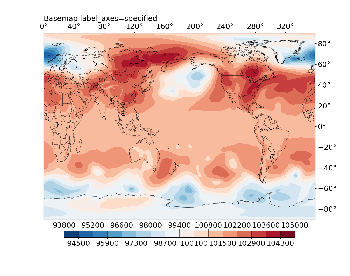
Fig. 12 Specify the axis ticks/ticklabels by setting label_axes = (0, 1, 1, 0). The 4 elements in the tuple correspond to the left, right, top, bottom sides, respectively.

Color for missing values

If not set, matplotlib sets the default background color to white, which also appears in many colormaps (e.g. the plt.cm.RdBu_r used as default colormap of gplot). Therefore it is easy to confuse your audience with the missing values and valid data values that happen to be represented with white color (or something very close to white). See the comparison below:

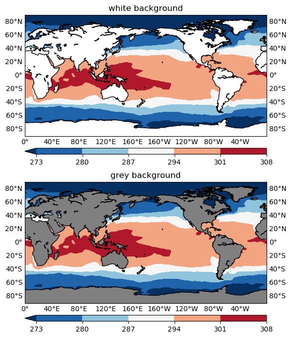
Fig. 13 Comparison of the missing values as represented with a white background (top) and grey background (bottom).

Therefore, to avoid such ambiguities, the missing values are represented by fill_color in gplot, using:

self.ax.patch.set_color(self.fill_color)

where fill_color is a keyword argument to the __init__ method of base_utils.Plot2D and base_utils.plot2(). It is defaulted to a grey color (0.8).

Font size

The font sizes are controlled by the fontsize keyword argument to the __init__ method of base_utils.Plot2D and base_utils.plot2(). It is defaulted to 11, and affects the sizes of these texts in a plot:

• title

• axes ticklabels

• axes labels

• colorbar ticklabels and units

• reference quiver key units

When the figure has more than 1 subplots, the font sizes are adjusted by the following empirical formula:

\[s_{adj} = \frac{7}{MAX\{n_r, n_c\}} + s_0\]

where:

• \(s_0\) is the fontsize argument (default to 11).

• \(n_r, n_c\): the number of rows, columns in the subplot layout.

• \(s_{adj}\): the adjusted font size for the subplot.

Default parameters

gplot defines the following dictionary of default parameters:

# Default parameters
rcParams = {
    'legend': 'global',
    'title': None,
    'label_axes': True,
    'axes_grid': False,
    'fill_color': '0.8',
    'projection': 'cyl',
    'legend_ori': 'horizontal',
    'clean': False,
    'bmap': None,
    'isgeomap': True,
    'fix_aspect': False,
    'nc_interface': 'cdat',
    'geo_interface': 'basemap',
    'fontsize': 11,
    'verbose': True,
    'default_cmap': plt.cm.RdBu_r
}

The base_utils.rcParams dict can be altered to make a change persistent in a Python session. And the base_utils.restoreParams() can be used to restore the original values. E.g.

gplot.rcParams['fontsize'] = 4

test_basemap_default()
test_basemap_isofill_overflow()

gplot.restoreParams()

test_basemap_isolines()