Basic plots
Table of Contents
Overall design of gplot
The overarching structure of gplot is pretty simple (see Fig.2): there are 2 major plotting classes, Plot2D and Plot2Quiver. The latter is specifically for 2D quiver plots, and the former handles commonly used 2D visualization types, including
isoline/contour
isofill/contourf
boxfill/imshow/pcolormesh
hatching
These 2 classes accept ndarray as inputs, which can be provided by 4 widely used netCDF file I/O modules: netcdf4, CDAT, Iris and xarray. Note that these are optional dependencies, and both Plot2D and Plot2Quiver work for plain ndarray data as well.
Note
Only netcdf4 and CDAT are currently supported. For the latter, only its cdms2 module is required.
On top of Plot2D and Plot2Quiver, plotting with geographical map projections are supported by utilizing basemap or Cartopy, giving rise to 4 derived classes:
Plot2Basemap: 2D plots as Plot2D but using basemap as the “backend” for geographical map projections.
Plot2QuiverBasemap: 2D quiver plots as Plot2Quiver but using basemap as the “backend” for geographical map projections.
Plot2Cartopy: 2D plots as Plot2D but using Cartopy as the “backend” for geographical map projections.
Plot2QuiverCartopy: 2D quiver plots as Plot2Quiver but using Cartopy as the “backend” for geographical map projections.
Note
basemap has been deprecated, however, Cartopy is not fully mature in terms of features and robustness. In gplot, more attention is paid on basemap plots, and the Cartopy counterparts are largely work-in-process at the moment.
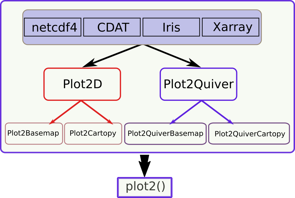
Fig. 2 Overarching structure of gplot.
Basic plotting syntax
To give an example of using Plot2Basemap:
figure = plt.figure(figsize=(12, 10))
ax = figure.add_subplot(111)
iso = gplot.Isofill(var)
gp = Plot2Basemap(var, iso, lons, lats, ax=ax)
gp.plot()
figure.show()
where:
varis thendarrayinput data to be plotted.isois anIsofillobject, which defines an isofill/contourf plot. More details onIsofillare given in Create isofill/contourf plots.lonsandlatsgive the longitude and latitude coordinates, respectively. They define the geographical domain to generate the map.
This also illustrates the basic “syntax” of gplot’s plotting function: there are 3 major elements that define a plot:
var: the input array – what to plot,iso: the plotting method – how to plot, andax: the matplotlib axis object – where to plot.
Similarly, for a 2D quiver plot example:
figure = plt.figure(figsize=(12, 10))
ax = figure.add_subplot(111)
q = gplot.Quiver(step=8)
pquiver = Plot2QuiverBasemap(u, v, q, xarray=lons, yarray=lats,
    ax=ax, projection='cyl')
pquiver.plot()

figure.show()
Note that in this case, there are 2 input arrays (u and v), the u- and
v- velocity components. And q = gplot.Quiver(step=8) defines the plotting
method.
With these 3 basic elements – input array, plotting method and axis – provided, gplot will try to handle the remaining trifles for you, including the axes ticks and labels, colorbar, subplot numbering etc..
Lastly, there is also a plot2() interface function in gplot that wraps
everything in a single function call. To reproduce the 1st example above, one
can use:
figure = plt.figure(figsize=(12, 10))
ax = figure.add_subplot(111)
iso = gplot.Isofill(var)
gplot.plot2(var, iso, ax, xarray=lons, yarray=lats)
figure.show()
And the 2nd example can be achieved using:
figure = plt.figure(figsize=(12, 10))
ax = figure.add_subplot(111)
q = gplot.Quiver(step=8)
gplot.plot2(u, q, ax, xarray=lons, yarray=lats, var_v=v,
    projection='cyl')
figure.show()
Note that the v- component has been provided using the var_v keyword argument.
These design choices are taken to achieve the primary goal of gplot, which is to help create good enough plots as quickly and easily as possible.