Create isoline/contour plots
Table of Contents
The Isoline class
To create an isoline/contour plot, one creates a base_utils.Isoline
object as the plotting method, and passes it to the base_utils.Plot2D
constructor or the base_utils.plot2() function.
In many aspects, the base_utils.Isoline class is similar as
base_utils.Isofill (it is in fact derived from the latter).
They share these arguments in their __init__() methods:
varsnumzerosplitlevelsmin_levelmax_levelqlqrvcentercmap
More explanations of these arguments are given in Create isofill/contourf plots.
There are a few arguments unique to Isoline, and are introduced below.
Line width and color controls
Line width is controlled by the line_width input argument, which is default
to 1.0.
See Fig.5b for an example of changing the line width to a
larger value.
Line color, by default, is determined by the colormap (cmap).
Alternatively, one can use only the black color by specifying black = True.
Or, use a different color for all contour lines color = 'blue'.
For single colored isoline plots, the colorbar will not be plotted.
See Fig.5b,c,d for examples of monochromatic isoline plots.
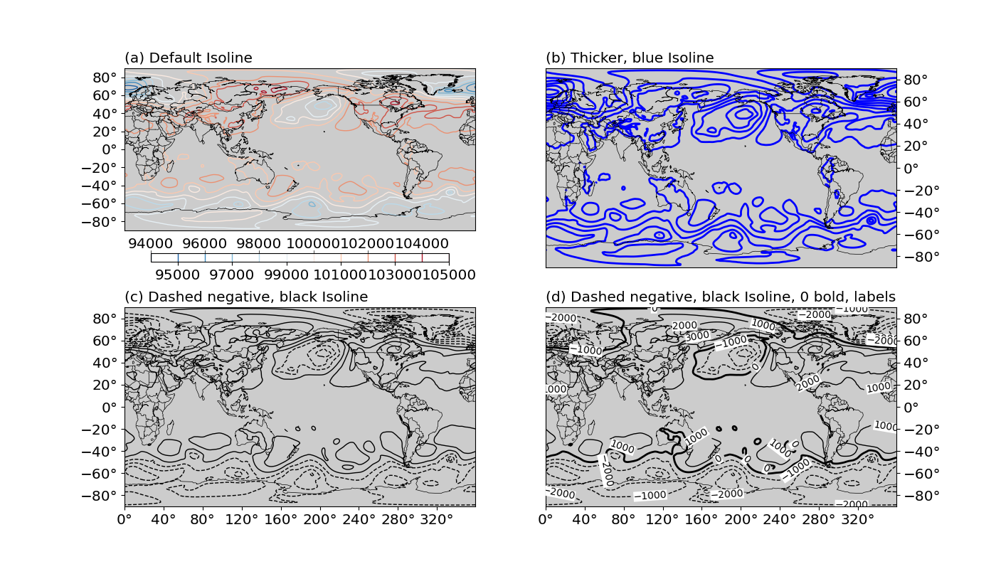
Fig. 5 Isoline plot examples. Complete script can be found in tests.basemap_tests.test_basemap_isolines()
(a) default isoline plot: colored contours, linewidth=1.
(b) isoline plot with linewidth=2.0, color='b'.
(c) isoline plot with black=True, dash_negative=True.
(d) isoline plot with black=True, dash_negative=True, bold_lines=[0,], label=True, label_box=True.
Use dashed line for negatives
It is also common to use dashed lines for negative contours and solid lines for positive ones, with optionally a 0-level contour as bold. These can be achieved using:
isoline = gplot.Isoline(var, 10, zero=1, black=True, dash_negative=True,
                        bold_lines=[0,])
See Fig.5c,d for examples.
Note
It is possible to set multiple levels as bold, by specifying them in a list
to bold_lines.
Label the contour lines
For plots with monochromatic contour lines, one needs to provide a different mechanism
for the reading of contour levels, such as labelling out the contours. This can
be achieved by passing in the label = True argument.
The format of the labels can be controlled by label_fmt. If left as label_fmt = None,
it will use a default Formatter.
An optional bounding box can be added by label_box = True, and one can
change the box background color by altering label_box_color.
See Fig.5d for an example.
The mappable object
gplot calls matplotlib’s (or basemap’s, if it is using Plot2Basemap)
contour() function under the hood. The function returns a mappable object,
e.g. cs = plt.contour(data). This mappable object is stored as
an attribute of the base_utils.Plot2D (or
basemap_utils.Plot2Basemap) object:
>>> plotobj = Plot2Basemap(var, iso, lons, lats, ax=ax)
>>> plotobj.plot()
>>> plotobj.cs
<matplotlib.contour.QuadContourSet object at 0x7f0e3e6b4550>
The same plotobj is returned by the base_utils.plot2() function,
therefore, the mappable object can be retrieved using:
>>> pobj = gplot.plot2(var, iso, ax, xarray=lons, yarray=lats)
>>> pobj.cs
<matplotlib.contour.QuadContourSet object at 0x7f0e3e6b4550>