Create quiver plots
Table of Contents
The Quiver class
To create a 2D quiver plot, one creates a base_utils.Quiver
object as the plotting method, and passes it to the base_utils.Plot2Quiver
constructor or the base_utils.plot2() function.
The __init__() of base_utils.Quiver takes these input arguments:
stepresoscalekeylengthlinewidthcoloralpha
linewidth, color and alpha should be self-explanatory. Others are explained
in further details below.
Control the quiver density
When the input data have too fine a resolution, the quiver plot may end up being too dense and not quite readable (see Fig.8a below for an example). This can be solved by either
sub-sampling the data with a step:
u = u[::step, ::step]; v = v[::step, ::step], orregridding the data to a lower resolution
reso.
Method 1 is controlled by the step input argument (see Fig.8b below for an example), and the latter method the reso argument
(see Fig.8c,d). If both are given, the
latter one takes precedence.
Note
regridding requires scipy as an optional dependency.
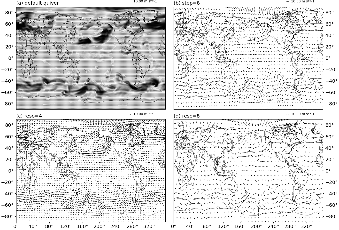
Fig. 8 Density control of a quiver plot.
(a) default quiver density q = Quiver().
(b) reduced density by sub-sampling: q = Quiver(step=8).
(c) reduced density by regridding: q = Quiver(reso=4).
(d) reduced density by regridding: q = Quiver(reso=8).
Control the quiver lengths
The lengths of the quiver arrows are controlled by the scale argument. A
larger scale value creates shorter arrows. When left as the default None,
it will try to derive a suitable scale level for the given inputs.
The length of the reference quiver arrow is controlled by the keylength
argument. Given a set scale, a larger keylength makes the reference
quiver arrow longer. Similar as scale, keylength is default to
None, and the plotting function will try to derive a suitable value
automatically for you.
Fig.9 below shows some examples of controlling the lengths.
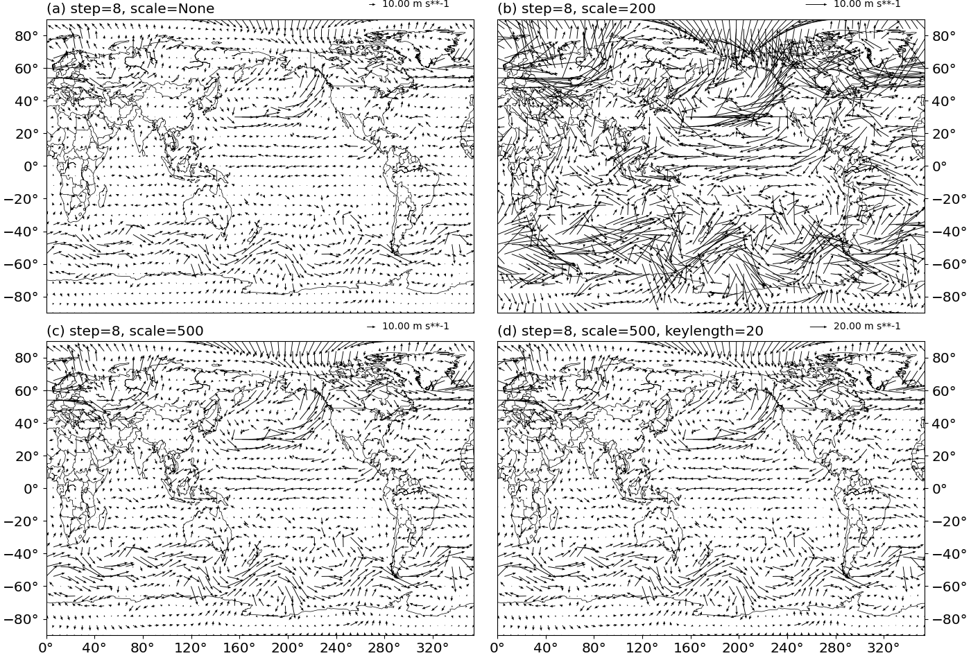
Fig. 9 Length control of a quiver plot.
(a) automatic scale q = Quiver(step=8, scale=None).
(b) specify scale=200: q = Quiver(step=8, scale=200).
(c) specify scale=500: q = Quiver(step=8, scale=500).
(d) specify scale=500, keylength=20: q = Quiver(step=8, scale=500, keylength=20).
Quiver overlay
It is common to see quiver plots superimposed on top of an isofill/contourf plot.
To achieve this, simply re-use the same axis object in the isofill/contourf
plot, and the subsequent quiver plot. E.g.
figure = plt.figure(figsize=(12, 10), dpi=100)
ax = figure.add_subplot(111)
iso = gplot.Isofill(var1)
q = gplot.Quiver(reso=5, scale=500)

gplot.plot2(var1, iso, ax, projection='cyl')
gplot.plot2(u, q, var_v=v, xarray=lons, yarray=lats,
            ax=ax, title='quiver overlay', projection='cyl')
figure.show()
The result is given in Fig.10 below.
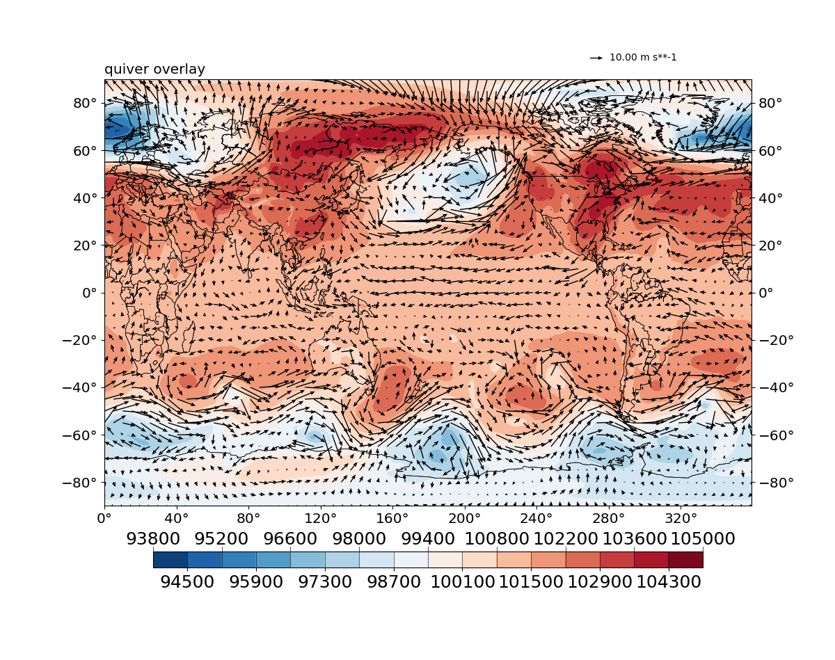
Fig. 10 Quiver plot on top of isofill.
Curved quiver plots
Sometimes one needs to visualize a vector field in a region where the vector
magnitudes are rather small, and a larger domain is needed to be shown at the
same time to give enough context. In such cases, when the scale is adjusted
to a comfortable value for the target region to be readable, other regions may
have quiver arrows that are too large and the plot looks messy.
One possible solution is to use curved quivers rather than straight ones.
matplotlib does not support this out-of-the-box, some hacks are used to
achieve this. Due credits to the author of this repo, and this stackoverflow
answer.
A curved quiver plot is done by passing in curve=True, e.g.:
figure = plt.figure(figsize=(12, 10), dpi=100)
ax = figure.add_subplot(111)
q = gplot.Quiver(step=8)
pquiver = Plot2QuiverBasemap(
    u, v, q, xarray=lons, yarray=lats, ax=ax, title='curved quiver',
    projection='cyl', curve=True)
pquiver.plot()

figure.show()
The result is given in Fig.11 below.
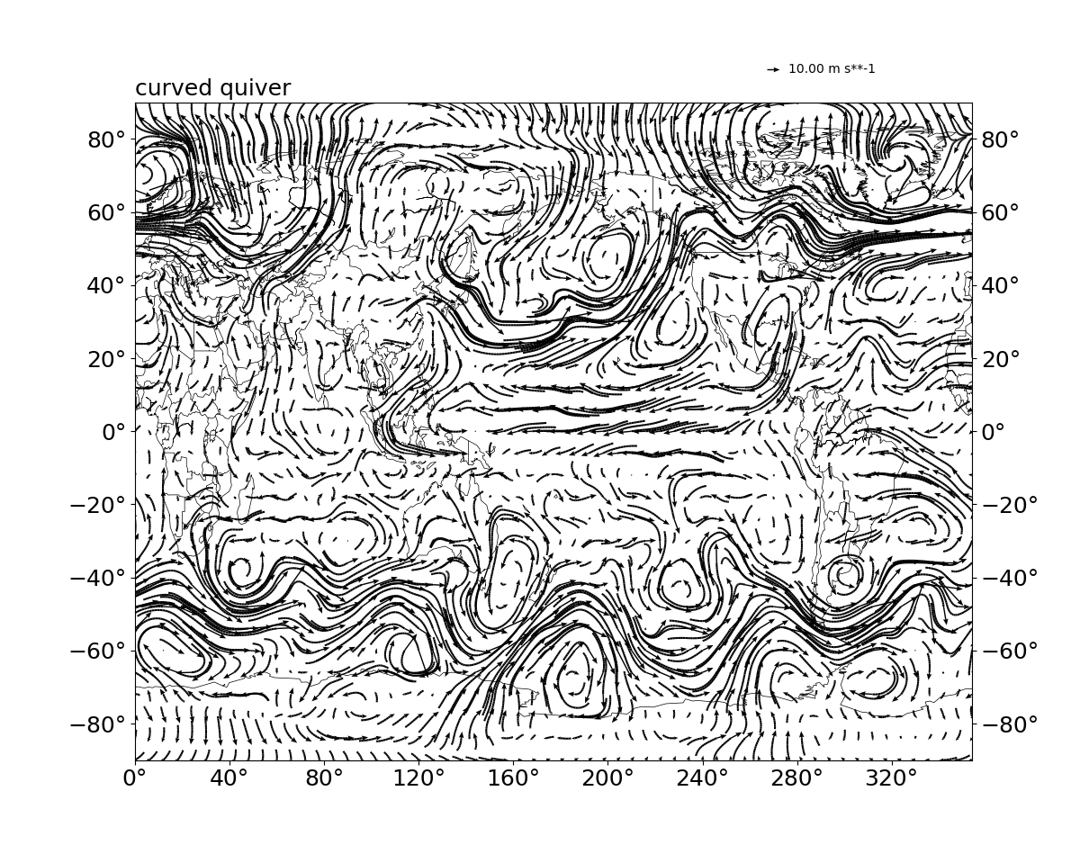
Fig. 11 Curved quiver plot.
Note
Curved quiver plot takes notably longer to generate, and is considered experimental at the moment.
The mappable object
The mappable object of a quiver plot is stored as an attribute of the
base_utils.Plot2Quiver (or
basemap_utils.Plot2QuiverBasemap) object:
>>> q = gplot.Quiver()
>>> pobj = Plot2QuiverBasemap(u, v, q, xarray=lons, yarray=lats, ax=ax, projection='cyl')
>>> pobj.plot()
>>> pobj.quiver
<matplotlib.quiver.Quiver object at 0x7f2e03aed750>